You built a beautiful model. The R-squared looks great, the variables make sense, and you're ready to predict next quarter's stock returns or real estate prices. You hit enter, get your forecast, and place your bet. Then the market does something completely wild, and your prediction is off by a mile. Sound familiar? The culprit, more often than not, is a statistical gremlin called heteroskedasticity. It's not a fancy word to impress people at parties. It's the reason your confidence intervals are lies and your risk estimates are fantasies.
Let me put it simply. Most basic models assume the "noise" or error in your data is consistent. Like a steady hum in the background. Financial data doesn't hum. It screams and whispers. Think of the calm of a 2017 market versus the sheer panic of March 2020. The volatility—the size of the ups and downs—changes. That's heteroskedasticity in action: the variance of the errors is not constant. Ignoring it means your model is wearing blinders during a hurricane.
Your Quick Guide to Navigating This Article
What Heteroskedasticity Really Means (For Your Portfolio)
Textbooks define it as "non-constant variance of the error terms." Let's translate that to money. You're modeling the daily returns of a tech stock. Some days, it moves 0.5%. Other days, after an earnings report, it jumps 8%. The "error" in your model—the part you can't explain with your factors—has a much bigger range on earnings day. The variance isn't constant; it clusters.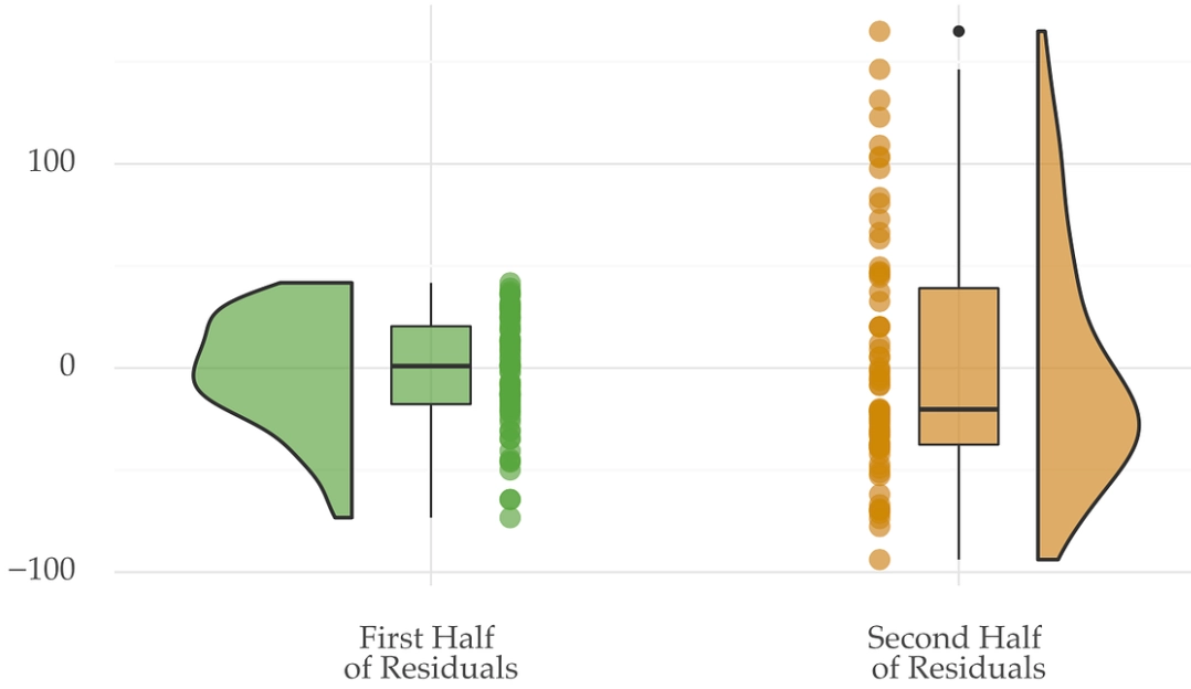
This clustering is often called volatility clustering, and it's the most common face of heteroskedasticity in finance. Quiet periods follow quiet periods. Turbulent periods follow turbulent periods. Robert Engle won a Nobel Prize for formalizing this idea with ARCH/GARCH models. The key insight for you is this: assuming constant variance when it's not leads to two massive, concrete problems.
The Two Costs of Ignoring It
1. Inefficient Estimates: Your model's coefficients (the betas telling you how much Y changes with X) aren't as precise as they could be. It's like using a blurry ruler.
2. The Bigger Sin: Misleading Inference. This is where you get hurt. Your software calculates standard errors and p-values assuming that steady hum. When volatility clusters, those standard errors are wrong. Often, they're too small. You end up thinking a variable is statistically significant (e.g., "this economic indicator truly predicts returns!") when, in reality, the evidence is flimsy. You're overconfident. You see a signal in the noise and bet real money on a mirage.
I learned this the hard way early in my career, building a model linking trading volume to price swings. The stats looked solid—until I plotted the residuals. They fanned out dramatically as volume increased. The model was useless for high-volume days, precisely when I needed it most. The standard tests had missed the severity because I hadn't looked at the picture.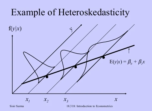
How to Spot the Signs Before It's Too Late
You don't need a PhD to check for this. The first and best tool is your eyes.
The Residual Plot: After you run any regression model, plot the residuals (the prediction errors) on the y-axis. On the x-axis, plot either the predicted values or the time sequence. What you want to see is a random scatter, a cloud of points with no pattern. What you often see in finance is one of these red flags:
- The Fan (or Funnel): The spread of residuals gets wider as the predicted values increase. Common in cross-sectional data (e.g., the variance of forecast errors is larger for big-cap stocks than small-cap stocks).
- The Volatility Cluster: In time-series data, you'll see periods where all the residuals are small and tight, followed by periods where they're large and wild. Look at a plot of stock market returns—the clusters are obvious.
After the visual check, use a formal test. The Breusch-Pagan test is the classic. The White test is a more general version. Most statistical packages run these in one line of code. Here’s the practical cheat sheet:
| Method | What It Does | Best For | Quick Tip |
|---|---|---|---|
| Eye Test (Residual Plot) | Visual pattern detection | Initial screening, understanding the nature of the problem | Always do this first. No test can replace a good plot. |
| Breusch-Pagan Test | Tests if variance depends on model's independent variables | Cross-sectional data, detecting "the fan" | Simple and direct. A low p-value ( |
| White Test | A more robust version of Breusch-Pagan | When you suspect more complex relationships | Less prone to misspecification, but slightly more complex. |
| ARCH-LM Test | Specifically tests for autoregressive conditional heteroskedasticity | Financial time-series, volatility clustering | The go-to test if you're working with daily returns or any asset price series. |
A word of warning: these tests are sensitive. In large samples, they might flag trivial heteroskedasticity that isn't practically important. The visual impact matters more. If your plot looks okay but the test p-value is 0.04, the economic significance might be minimal. If your plot looks like a shotgun blast, you have a problem regardless of the p-value.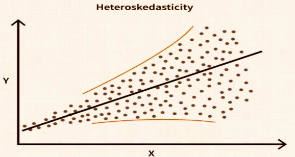
Fixing the Problem: From Quick Patches to Advanced Solutions
Okay, you found it. Now what? The solution depends entirely on your goal. Are you just trying to get reliable p-values for your research report? Or are you building a trading system to forecast volatility itself?
The Quick Fix: Robust Standard Errors
This is your first line of defense. You don't change your model's coefficients; you just recalculate the standard errors in a way that's robust to heteroskedasticity. In Python's statsmodels, you add cov_type='HC3' to your regression. In R, use coeftest with vcov = vcovHC.
This method, often called Heteroskedasticity-Consistent Standard Errors (HCSE) or White standard errors, is like putting better shock absorbers on your car. The road (data) is still bumpy, but your reading of the gauges (significance tests) is now stable. Use this when your primary concern is valid inference—making sure you're not fooled by false significance.
It's a patch, not a cure. Your predictions are still made with the original, potentially inefficient model.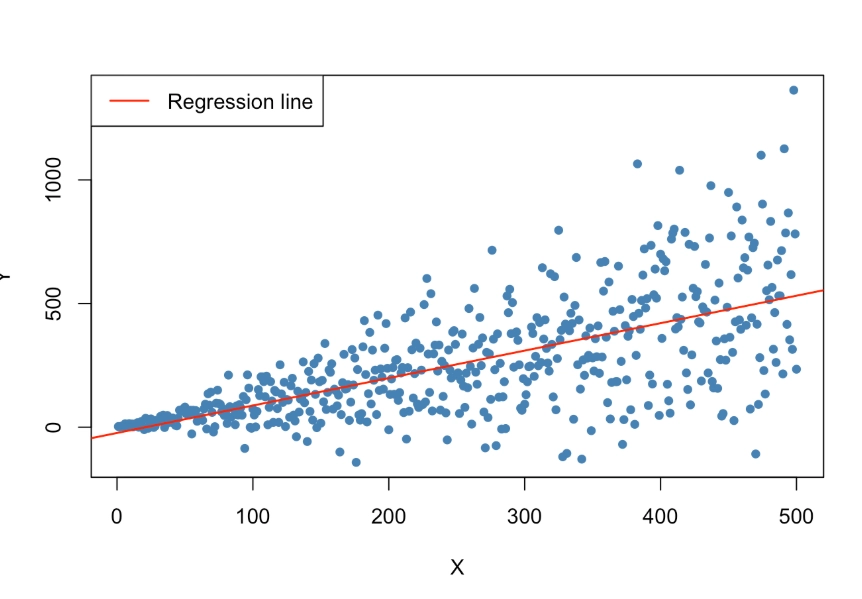
The Model Transformation
Sometimes you can transform your dependent variable. If you're dealing with percentages or amounts where errors grow with size, using the logarithm can often stabilize the variance. This is common when modeling prices, market capitalization, or income data. It's not a universal fix, but it's a good trick to have in your toolkit.
The Power Tool: GARCH Models
If you're in finance and your goal is to model and forecast volatility, this is the main event. GARCH (Generalized Autoregressive Conditional Heteroskedasticity) models don't just correct for heteroskedasticity; they treat changing volatility as the phenomenon to be studied and predicted.
Think of it this way: a regular model says, "The return today is X + error." A GARCH(1,1) model says, "The return today is X + error, AND the variance of today's error depends on yesterday's error squared and yesterday's variance." It directly models the volatility clustering.
Where you use it: Value-at-Risk (VaR) calculations, options pricing (volatility is a key input), algorithmic trading strategies that adapt to market regimes, and any risk management dashboard that needs a dynamic volatility estimate.
Implementing GARCH is more involved. You'll use libraries like arch in Python. The payoff is a model that doesn't assume a calm world, but one that recognizes markets breathe in and out.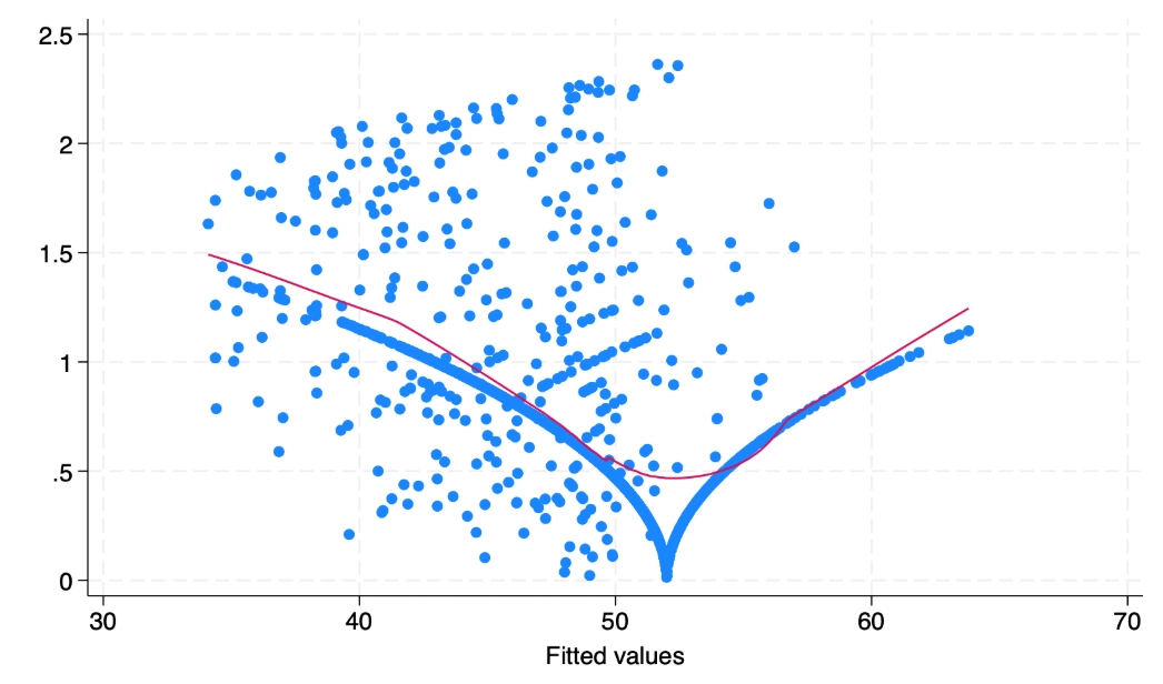
Putting It Into Practice: A Realistic Action Plan
Let's make this actionable. Here’s a step-by-step workflow you can apply to your next project.
- Build your initial model. Run your linear regression, your time-series model, whatever it is.
- Plot the residuals. Against predictions and against time. Stare at the plot. Is it a random cloud or does it tell a story?
- Run a formal test. For time-series, use the ARCH-LM test. For cross-section, use Breusch-Pagan or White.
- Choose your remedy based on goal:
- Goal: Reliable hypothesis testing. → Re-run your model with Robust Standard Errors (HCSE). Report these results.
- Goal: Forecasting the mean (e.g., future price). → Consider transformations (like logs) or using HCSE. Evaluate if the heteroskedasticity severely hurts prediction accuracy on new data.
- Goal: Forecasting or understanding volatility. → You need a GARCH-type model. This is a separate modeling project focused on variance.
- Validate. Check the residuals of your *corrected* model. The plots should look better. The tests should be cleaner.
Let's look at a tiny case study. I pulled S&P 500 daily returns for 2023. A simple model trying to predict today's return from yesterday's is basically useless (no surprise). But the residuals? They show clear quiet and loud periods. The ARCH-LM test p-value is effectively zero. For this data, if I wanted to forecast tomorrow's volatility for risk management, ignoring heteroskedasticity would be professional malpractice. A GARCH model is the only serious tool for the job.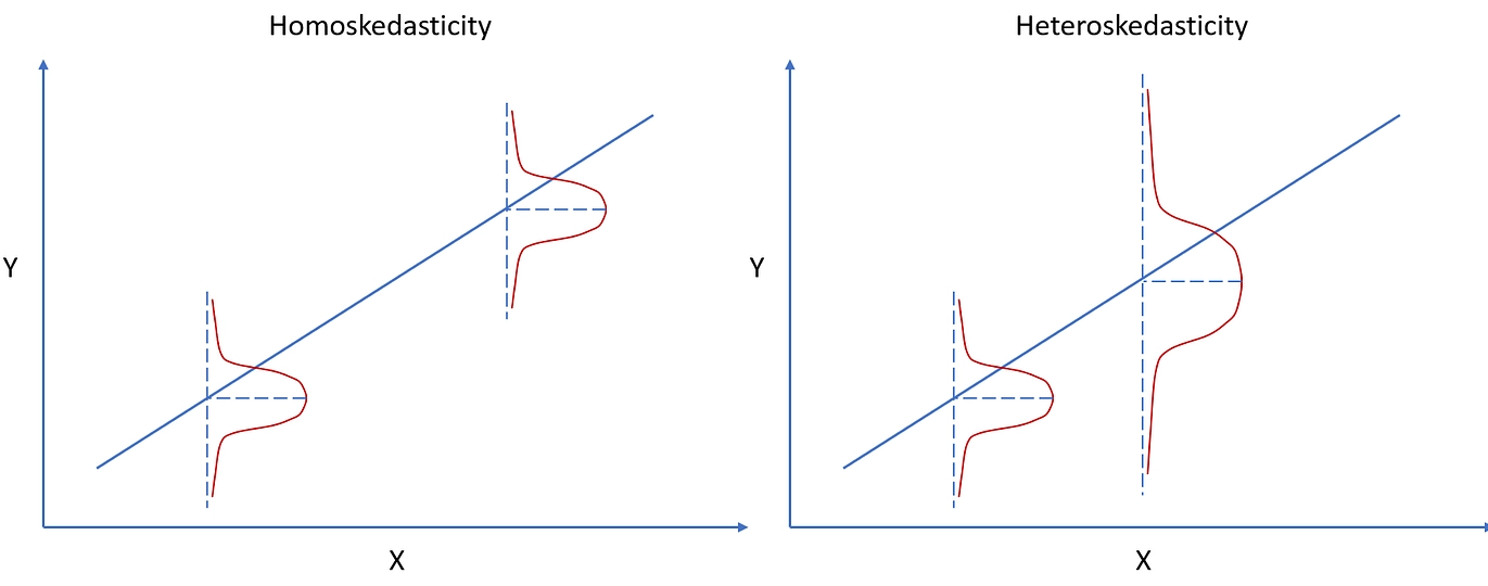
Questions You're Probably Asking
How can I quickly check for heteroskedasticity in my stock return data?
Plot the residuals from your model against the predicted values or against time. If you see a pattern like a fan or funnel shape, or clusters of high and low volatility, that's a visual red flag. Then, run a formal test like the Breusch-Pagan test, which is widely available in statistical software like Python's statsmodels or R. Don't just rely on the test p-value; always look at the plot first. The eye can catch patterns that a single test statistic might miss.
Is using a GARCH model the only way to handle heteroskedasticity for trading?
No, it's the most sophisticated way for volatility forecasting, but not the only one. For simpler tasks like improving regression coefficient estimates, using Heteroskedasticity-Consistent Standard Errors (HCSE) is often sufficient and easier. It doesn't model volatility, but it corrects your confidence intervals so you don't make false inferences. Think of HCSE as a defensive patch and GARCH as a full offensive strategy for predicting volatility itself. The choice depends on whether your goal is robust inference or active volatility prediction.
Can heteroskedasticity ever be beneficial or useful in financial analysis?
This is a great question most textbooks ignore. Yes, its presence is the entire foundation of volatility trading. Options pricing models, like Black-Scholes, rely on an estimate of future volatility. Traders who can better model changing volatility (heteroskedasticity) through tools like GARCH can identify mispriced options. So, while it's a nuisance for simple linear predictions, it's the raw material for complex strategies in derivatives markets. The problem isn't its existence; it's ignoring it when your model assumes it's not there.
The bottom line is this. Heteroskedasticity isn't a theoretical curiosity. It's the default state of financial markets. Treating it as a nuisance to be patched with robust errors is fine for one-off analysis. But to truly understand market risk and opportunity, you need to embrace it. Model it. The models that pretend the world is simple get left behind by the ones that acknowledge its beautiful, chaotic complexity.
Reader Comments